

Grids
Several kinds of finite element grids are implemented in JOREK. Some grids are used for the determination of the equilibrium only and are not aligned to the magnetic flux surfaces. These initial grids are (names of subroutines given):
grid_bezier_square: Rectangular grid in R- and Z-directionsgrid_polar_bezier: Polar grid with an adjustable boundary shape. Refer to Figure 1 and Figure 2 (grey). This is usually the default choice as initial grid.grid_bezier_square_polar: Combination of both, i.e., a square grid inside and a polar grid around it.
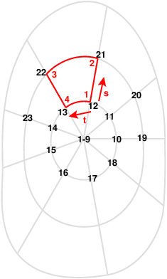
Figure 1: Example polar grid generated with grids/grid_polar_bezier.f90. The numbering scheme for the element's nodes is also shown with the numbering starting at the axis and the first elements sharing the axis node. Additionally, the s,t directions and order of the vertices are shown for one element in red.
As soon as the equilibrium has been determined, a finite element mesh can be generated that is aligned to the equilibrium magnetic flux surfaces. For this purpose, two grid generation routines are available:
grid_flux_surface: Two sides of the elements are aligned to the closed flux surfaces of a tokamak configuration without X-point (red in Figure 2, left).grid_xpoint: The elements are aligned to the flux surfaces of an X-point configuration with a single lower X-point (red in Figure 2, right).grid_double_xpoint: This routine is used for several things. It is used for upper single null configurations as well as for configurations that include two x-points inside of the computational domain of interest. These x-point pair can, but does not have to, form a symmetric double null.
In Figure 2, two finite element grids are shown. The grey mesh is of grid_polar_bezier type and used for the equilibrium determination only (initial grid). The flux-surface aligned grid for X-point geometry (grid_xpoint) that is successively used for the time-integration of the MHD-equations is shown in red.
The numbering of the nodes in polar and flux surface grids (black numbers), the numbering of the nodes within an element (red numbers) and the directions of the element-local coordinates $s$ and $t$ are shown.
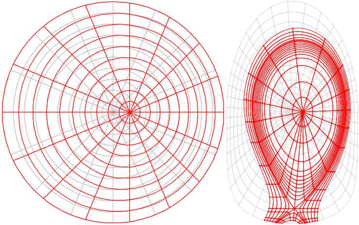
Figure 2: (left): Example flux-surface aligned grid constructed with grids/grid_flux_surface.f90. (right): Example X-point grid constructed with grids/grid_xpoint.f90. This requires a map of the poloidal magnetic flux from an existing polar grid (shown in gray). Actual applications require much higher resolution.
Tutorials
Here is a tutorial for the construction of basic X-point grids, double X-point grids, and wall-extended grids:
- Grad-Shafranov Tutorial
- X-point Grid Construction
- Double X-point Grid Construction
- Wall-extended Grid Construction
- Alternative wall-extended Grid Construction
- Gn-continuous Grid Construction