JOREK Solver

The implicit time integration scheme implemented by JOREK leads to a large and sparse linear system of the general form

\[A\,x = b.\]

The matrix $A$ is assembled in a distributed block-COO format (which can be converted to a distributed block-CSR format on demand) and is partitioned by toroidal Fourier harmonics and finite-element nodes. The solver infrastructure exploits this block structure at both the factorisation and the preconditioning level.

Two high-level solution strategies are supported:

	Direct solve	Iterative solve
Input flag	`gmres = .false.`	`gmres = .true.`
Method	Sparse LU factorisation of $A$	GMRES (or BiCGSTAB) with block preconditioner
Strengths	Robust; insensitive to conditioning	Lower memory; scales to large problems
Weaknesses	Memory and fill-in grow rapidly	Convergence depends on preconditioner
Typical use	Small-to-moderate problems	Large / production runs

Both strategies support multiple third-party libraries as back-ends and can optionally offload the matrix–vector products to GPU hardware.

The main entry point is solve_sparse_system() in solvers/mod_sparse.f90.

Direct Solvers

When gmres = .false. in the input file, the system is passed directly to one of the supported sparse-direct libraries. The library is selected at compile time via flags (USE_MUMPS, USE_PASTIX, USE_STRUMPACK) and at runtime by the corresponding use_* input flags.

Hint: Factorization of large sparse matrices is an expensive operation and will create a lot of fill-in resulting in increased memory requirements. Thus, for most cases use of the iterative solver is recommended!

Iterative Solvers

When gmres = .true., a Krylov iterative method is used, preconditioned by the block harmonic preconditioner described in the next section.

GMRES

Left-preconditioned restarted GMRES is implemented in solvers/mod_gmres.f90. (A more modern implementation avaliable in selected branches is implemented in solvers/mod_gmres2.f90).

The algorithm applies the preconditioner $M^{-1}$ to both the initial residual and to each new Krylov vector. Orthogonalisation is performed by a Gram–Schmidt variant (classical or modified, with or without re-orthogonalisation, controlled at compile time). Givens rotations maintain the upper Hessenberg in triangular form in-place. After each restart the solution is updated as $x \leftarrow x + V y$, where $y$ minimises the preconditioned residual over the current Krylov subspace.

Convergence is declared when

\[\frac{\|r_k\|}{\|r_0\|} < \texttt{gmres_tol}\]

or when the absolute residual drops below a secondary threshold.

Key input parameters:

Parameter	Default	Description
`gmres_m`	40	Restart dimension
`gmres_max_iter`	400	Maximum number of outer (restarted) iterations
`gmres_tol`	—	Relative residual tolerance

BiCGSTAB

BiCGSTAB (in solvers/mod_bicgstab.f90) is an alternative that requires no restart and uses $O(n)$ memory independent of the iteration count. It applies the preconditioner twice per iteration (once for the search direction, once for the stabilizer), which is more expensive per step than GMRES but avoids restarting costs. Enable it at compile time with the USE_BICGSTAB preprocessor flag.

Hint: Use of BiSCSTAB is generally not recommended.

Preconditioner

Preconditioning is essential in solving linear systems using iterative methods. The matrices resulting from the MHD formulations in JOREK are highly ill-conditioned and iterative methods do not converge without a proper preconditioner.
We choose a preconditioner$M$ such that we solve the modified left preconditioned system

\[M^{-1}A x = M^{-1}b,\]

where $M$ is "cheap" to invert and $M^{-1}A$ is a reasonably good approximation of the identity. There exist many "standard" techniques that can be applied to general systems without considering the original problem. These, of course, have the benefit of being "plug-and-play" and work reasonably well for a wide range of problems. When going into very ill-conditioned problems we find most of these approaches to have little to no effect. These cases require more advanced study to create tailored preconditioners to obtain good convergence.

The block harmonic preconditioner in JOREK exploits the toroidal Fourier structure of the MHD system to construct a preconditioner $M$ whose application requires only independent sparse-direct solves on smaller sub-systems, one per mode family.

The preconditioner is set up and applied by solvers/mod_preconditioner.f90.

Concept

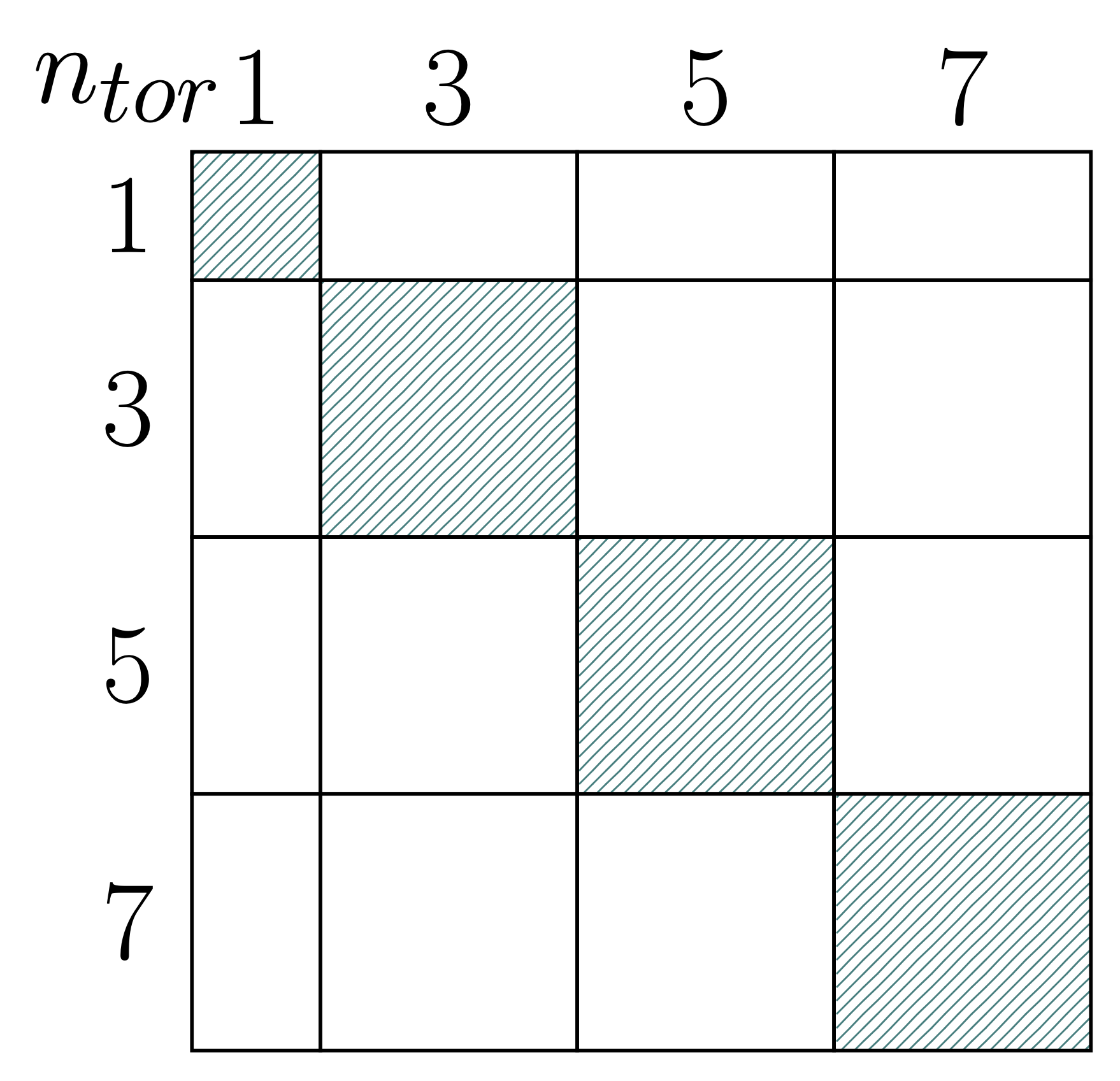
For a purely axisymmetric geometry, toroidal harmonics decouple completely: the mode-$n$ rows of the system matrix have no coupling to mode-$m \ne n$ columns. JOREK's matrix does contain inter-harmonic coupling terms (from inter-harmonic coupling terms in the system), but in many cases the dominant, physics-relevant coupling is intra-harmonic. The preconditioner $M$ is therefore built by grouping the toroidal modes into families and assembling one block-diagonal preconditioner matrix per family that retains all intra-family coupling while discarding the inter-family terms. Each mode family is then factorised independently by the selected direct-solver library.

Mode Family Distribution

Toroidal modes $0, 1, 2, 3, \ldots$ are partitioned into mode families. Two strategies are available:

Automatic (autodistribute_modes = .true.): mode 0 (axisymmetric) forms its own family; remaining modes are paired as $(n_1, n_2), (n_3, n_4), \ldots$
Manual: the user specifies n_mode_families, modes_per_family(:), and mode_families_modes(:,:) explicitly.

Overlapping Mode Families

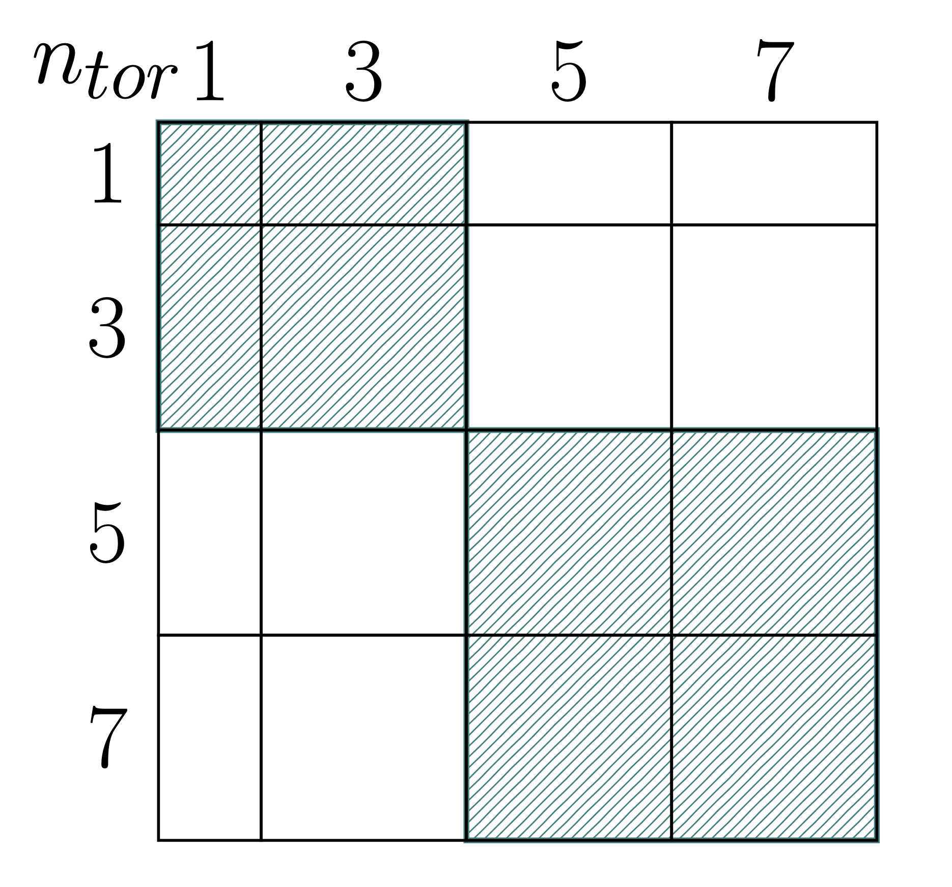
Manual families do not have to form a disjoint partition: the same toroidal mode can appear in more than one family. Couplings between all modes belonging to a family are retained in that family's preconditioner block, which can improve GMRES convergence when important inter-harmonic couplings would otherwise be discarded.

When families overlap, their solutions contain contributions to the same rows of the global solution vector. JOREK combines these contributions using the factor assigned to each family in weights_per_family. The weights should be chosen consistently with the overlap; in the example below every mode belongs to two families, so every family has weight $0.5$:

autodistribute_modes = .false.
n_mode_families = 5

modes_per_family = 1, 3, 4, 4, 2
mode_families_modes(1,:) = 1
mode_families_modes(2,:) = 1, 2, 3
mode_families_modes(3,:) = 2, 3, 4, 5
mode_families_modes(4,:) = 4, 5, 6, 7
mode_families_modes(5,:) = 6, 7

weights_per_family = 0.5, 0.5, 0.5, 0.5, 0.5

The values in mode_families_modes are the one-based i_tor mode indices used internally by JOREK. Increasing the number of modes per family retains more of the original matrix coupling, but also produces larger and more expensive blocks to factorise.

MPI ranks are distributed among families in the same way:

Automatic (autodistribute_ranks = .true.): ranks are distributed as equally as possible across families.
Manual: specified via ranks_per_family(:).

Because families can have very different block sizes, an equal rank distribution may give poor load balance. A useful starting heuristic is to assign ranks approximately in proportion to the square of the number of modes in each family. For the five overlapping families above, one possible setup is:

autodistribute_ranks = .false.
ranks_per_family = 2, 8, 16, 16, 4

The total number of MPI ranks used for the run must equal the sum of ranks_per_family. The optimal distribution depends on the matrix structure, the direct solver, and the machine, so this initial allocation may require tuning.

For further details, see Holod et al., Enhanced preconditioner for JOREK MHD solver, Plasma Physics and Controlled Fusion 63, 114002 (2021).

Single block harmonic — *Single harmonic pair per block*

Grouped block harmonic — *Grouped harmonic families*

Preconditioner Solve Workflow

Each GMRES / BiCGSTAB preconditioner application performs the following steps:

Scatter RHS — extract the rows belonging to this mode family from the global residual vector (via pre-computed row_index mapping).
Solve — the family's direct solver (MUMPS / PaStiX / STRUMPACK) factorises or reuses, and solves the preconditioner matrix for the local RHS.
Gather solution — contributions from all families are reduced by MPI_AllReduce (sum) into the global solution vector; each family's rows are weighted by row_factor (normally 1, or set from weights_per_family for manually defined families).

Factorisation Reuse

Refactoring the preconditioner at every time step is expensive. Thus, we can reuse the factorized preconditioner matrices over multiple timesteps, where they still provide a good approximation of the linear system. JOREK reuses the existing factorisation (the solve_only path) when:

\[\texttt{iter_gmres} + \texttt{iter_prev} \le 2 \times \texttt{iter_precon} \quad \text{and} \quad \texttt{n_since_update} < \texttt{max_steps_noUpdate}\]

where iter_precon and max_steps_noUpdate are input parameters. When neither condition is satisfied, the preconditioner matrix is reassembled and refactorised.

Preconditioner Matrix Assembly

Two assembly strategies are available (selected by compile-time flag DIRECT_CONSTRUCTION):

Direct construction: each MPI rank assembles its part of the preconditioner matrix directly at the finite-element level, without the distribution step.
Distributed construction: the full system matrix is communicated via MPI_ALLTOALLV to the rank groups that own each mode family, which then extract their rows locally.

PETSc Integration

Note: PETSc-based solver paths are under active development. This section will be expanded once the implementation stabilises.

When compiled with USE_PETSC, an alternative solver path is available that uses PETSc's KSP framework for both direct and iterative solves. The PETSc integration layer lives in solvers/mod_petsc.f90 and exposes:

A persistent KSP context that is reused across time steps.
An MPIBAIJ system matrix that can be filled from JOREK's native BCSR data.
Plug-in preconditioners implemented as PETSc PCSHELL or PCFIELDSPLIT objects.

Details of the PETSc-based preconditioners and their configuration will be documented separately.