

Types of boundary conditions
-
Dirichlet: The variable's value is kept constant over time (e.g. $\rho=cte$ or $\delta\rho = 0$)
-
Natural: A condition on the variable's normal derivative through a boundary integral term (e.g. $\nabla T\cdot\mathbf{n} = c T$). The implementation is explained in the JOREK overview article section 2.3.2. See also an example in "sheath boundary conditions for the heat-flux"
-
Special conditions: Special conditions can be applied to some variables. For example we typically set the parallel velocity to be the sound speed ($v_\parallel=c_s$) in the divertor region (the Mach=1 condition).
-
No explicit conditions: We can choose not to apply any boundary condition for the variable. For some variables this can cause the code to crash since the system is not determined (e.g. for $\psi$). However there are variables in which not applying explicitly a condition determines implicitly another one. For example for $\rho$ and $T$ not applying any condition directly implies that ($\nabla T\cdot\mathbf{n} = 0$ and $\nabla \rho\cdot\mathbf{n} = 0$), since is equivalent to implement a boundary term that is 0.
Types of boundaries (boundary type indices)
The JOREK boundary can be separated into different parts, for example the divertor targets (with finite $\mathbf{B}\cdot\mathbf{n}$) and the boundary which is aligned with the magnetic field ($\mathbf{B}\cdot\mathbf{n}=0$). To apply boundary conditions in different boundary regions, such regions are labeled with a "boundary type". This labeling depends on the grid that you choose, see below some examples (not complete)
- Polar grid (grid_polar_bezier): "2" for all the boundary
- Polar-aligned grid (grid_flux_surface): "2" for all the boundary
- X-point grid (grid_xpoint): "1" for the divertor targets, "2" for the flux-aligned boundary, "3" for the grid corners
Boundary types > 3 exist for more complex grids. You can check the boundary types that you use with jorek2_postproc and the command grid_diagnostics.
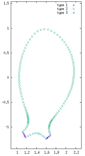
The plot was generated by using gnuplot and the following command:
p 'postproc/nodes_by_boundary_type_00000001_s00000.dat' t 'type 1', 'postproc/nodes_by_boundary_type_00000002_s00000.dat' t 'type 2', 'postproc/nodes_by_boundary_type_00000003_s00000.dat' t 'type 3'
Boundary types with patches
!!! RECAP !!! DEFINED BY GUIDO
- 1: TARGET, side 2
- 2: TANGENT, side 3
- 3: CORNER, between type-1 and type-2
- 4: TARGET, side 2 (Same as type-1)
- 5: TARGET, side 3
- 9: CORNER, between type-4 and type-5
!!! RECAP !!! DEFINED BY STAN TO INCLUDE FIELD DIRECTION, COMPATIBLE WITH OLD GRIDS
- 1: TARGET, side 2 (inward field)
- 11: TARGET, side 2 (outward field)
- 5: TARGET, side 3 (inward field)
- 15: TARGET, side 3 (outward field)
- 9: CORNER, free (inward field)
- 19: CORNER, free (outward field)
- 2: TANGENT, side 3 (tangent field)
- 12: TANGENT, side 2 (tangent field)
- 20: CORNER, fixed (tangent field)
- 21: CORNER, inverted (3 elements) (special case)
! NOT USED IN NEW GRID
- 3: Corner between type-1 and type-2 (only for old grid)
- 4: Same as type-1 (only for old grid)
!!! MAPPING !!! TO GO FROM STAN'S DEFINITION TO GUIDO'S
- 1 -> 1
- 11 -> 1
- 5 -> 5
- 15 -> 5
- 9 -> 9
- 19 -> 9
- 2 -> 2
- 12 -> not defined!
- 20 -> 9 (because not defined!)
- 21 -> not defined!
- 3 -> 3
Specifying the boundary conditions in the input file
The "bcs" structure allows you to add the boundary conditions in the input file. For example, to apply a Dirichlet BC for variable "rho" and boundary type "j", add the following to the input file:
bcs(j)%dirichlet%rho = .true.
IMPORTANT: Trying to specify a boundary condition for all boundary types with the following statement will not work:
bcs(:)%dirichlet%rho. You have to retype each line for each boundary type index separately:bcs(1)%dirichlet%rho=.t.,bcs(2)%dirichlet%rho=.t., etc.
IMPORTANT: If you want to apply any kind of natural boundary conditions, you must set
bc_natural_open=.t.in the input file.
Available boundary conditions
To see all available boundary conditions, see the table below for boundary type "i":
| Variable | Dirichlet | Natural (bc_natural_open=.t.) | Special | None applied |
|---|---|---|---|---|
| $\psi$ | bcs(i)%dirichlet%psi | None | free-boundary | ? |
| $u$ | bcs(i)%dirichlet%u | None | None | ? |
| $j$ | bcs(i)%dirichlet%zj | None | free-boundary | Determined by induction equation |
| $w$ | bcs(i)%dirichlet%w | None | None | ? |
| $\rho$ | bcs(i)%dirichlet%rho | bcs(i)%natural%rhoCondition: $D\nabla\rho\cdot\mathbf{n} = -r_\rho\rho\mathbf{v}\parallel \cdot\mathbf{n}$ with $r\rho$ = density_reflection | None | $\nabla\rho\cdot\mathbf{n}=0$ |
| $T$ | bcs(i)%dirichlet%T | bcs(i)%natural%Tsee here | None | $\nabla T \cdot\mathbf{n}=0$ |
| $T_i$ | bcs(i)%dirichlet%Ti | bcs(i)%natural%Tisee here | None | $\nabla T_i\cdot\mathbf{n}=0$ |
| $T_e$ | bcs(i)%dirichlet%Te | bcs(i)%natural%Tesee here | None | $\nabla T_e\cdot\mathbf{n}=0$ |
| $v_\parallel$ | bcs(i)%dirichlet%vpar | bcs(i)%natural%vparmach_one_bnd_integral=.t.Condition: $v_\parallel = c_s$ via penalization method | bcs(i)%mach1Condition: $v_\parallel = c_s$ | ? |
| $\rho_n$ | bcs(i)%dirichlet%rhon | bcs(i)%natural%rhonCondition: $D_n\nabla\rho_n\cdot\mathbf{n} = -r_{\rho_n}\rho\mathbf{v}\parallel \cdot\mathbf{n}$ with $r{\rho_n}$ = neutral_reflection | None | $\nabla\rho_n\cdot\mathbf{n}=0$ |
| $n_{RE}$ | bcs(i)%dirichlet%nre | None | None | ? |
Default values
-
$\psi, u, j, w, n_{RE}$: Dirichlet for all boundary types
- $\rho, T, T_i, T_e, \rho_n$:
- None applied for boundary types "1, 4, 5, 9, 11, 15, 19"
- Natural for boundary types "1, 4, 5, 9, 11, 15, 19" (if
bc_natural_open=.t.) - Dirichlet for all other boundary types
- $v_\parallel$:
- Special Mach=1 for boundary types "1, 3, 4, 5, 9, 11, 15, 19"
- Dirichlet for all other boundary types
Conflicts between boundary conditions
Conflicts can occur when specifying multiple conditions. For example, what happens if you specify both bcs(i)%dirichlet%vpar=.t. and bcs(i)%mach1=.t.? In such cases, the following priority order applies (1 = highest priority):
- Special conditions (e.g., free-boundary and Mach=1)
- Dirichlet conditions
- Natural conditions
- No explicit conditions
Example 1: Apply Mach=1 to $v_\parallel$
bcs(i)%mach1 = .t.
Example 2: Apply Dirichlet to $v_\parallel$
bcs(i)%mach1          = .f.
bcs(i)%dirichlet%vpar = .t.
Example 3: Apply natural conditions to $T$
bc_natural_open    = .t.    ! Switches on boundary integral calls
bcs(i)%dirichlet%T = .f.
bcs(i)%natural%T   = .t.
Example 4: Set no conditions to $\rho$
bc_natural_open      = .f.
bcs(i)%dirichlet%rho = .f.
bcs(i)%natural%rho   = .f.